CTFS Tutorials

• Tutorials: Top Level
• Server Use
• Growth changes
• Mortality changes
• Mortality vs. dbh
• Population Changes
• Biomass
• Growth vs. DBH
• ImageJ
• Plot maps
• Topography

Source file: http://ctfs.si.edu/ctfsdev/CTFSRPackageNew/files/tutorials/GrowthChange

Growth changes

The question addressed here is how growth has changed with time, in particular how species differ in growth changes. There are two alternative models described:

• Growth rate changing linearly with time
• Growth rate varying from census to census, but not following a consistent change

Both hypotheses will be tested running models with the R function lmer in the package lme4. You will need to install the package.

1. Formatting data

The calculations start with the full plot dataframes described at http://ctfs.arnarb.harvard.edu/Public/CTFSRPackage/help/RoutputFull.pdf. The BCI data can be downloaded from http://ctfs.arnarb.harvard.edu/bci/RAnalyticalTables after filling out the request form http://ctfs.arnarb.harvard.edu/webatlas/datasets/bci/.

In the CTFSRPackage, there are functions for loading data and calculating growth rates. The function individual_grow.table collects results from several other functions to calculate growth rates for individual trees and assemble them into a table in the format used by lmer. It is described in the Demography package.

The purpose is to create tables of growth rates for every tree in every census interval. Choose any diameter category, and any set of censuses you wish to work with. Here is an example for big trees at BCI (dbh ≥ 400), with all seven censuses included.

The table grate has one row per individual growth measurement, and includes the tree’s tag number, coordinates, species, and dbh at two time periods. The column census gives the census interval, so 1 means growth between census 1 and 2, and 2 means growth from census 2 to 3, etc. The column censusfact is the same, but as a factor variable instead of an integer. The time column is the mid-point of the interval over which growth was measured, centered on 1992. This is the format needed by lmer. The reason for centering time is that it is much better in linear regressions to have the x-axis near zero.

The argument rnd indicates that dbhs<50 mm are rounded down to 5-mm, necessary because saplings at BCI in 1982 and 1985 were measuring in 5-mm increments. The growth functions in the CTFS R Package handle this.

The other columns are

• LnSize: log(dbh1)
• incgr: growth increment (difference in dbh) per year
• LnGrowth: log of the growth rate, with negatives and zeroes converted to 0.1 (from the argument mingrowth in the function)
• CRGrowth: power transformation of the growth rate, with negatives maintained negative (exponent = 0.45).

The analyses are most cleanly done using the cube root of growth rate (CRGrowth), so no assumptions about negative growths are needed. You are welcome to try either untransformed growth increment (incgr) or the log of growth (LnGrowth).

2. Mean forest-wide growth

First find the mean growth rate of all individuals in each census period using the table grate.

Calculate mean growth increment per census interval, and the mean(incgr) and mean(CRGrowth). These are simply the observed mean growth rates in all 6 census intervals. The time, meanyr, is the mean years since 1992 of each census interval.

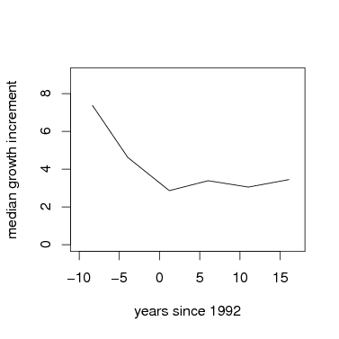
Graph mean growth vs. time. In this example, I use the mean of the cube-root of growth, but cube it to return to the original scale. You could also simply graph the mean growth increment.

3. Mixed model to assess species variation in linear changes through time

The function lmer runs a linear regression of growth rate vs. time, with species as a random effect. This is equivalent to a hierarchical model, where a Gaussian distribution describes the variation in species responses. The cube root of growth is used as the response, in order to come closer to a normal error term (required in textitlmer) while not requiring artificial exclusion of negative growth rates (as a log-tranformation would).

Since BCI growth rates declined over the first 3 censuses, but have not changed since, I chose to run separate models for census ≤ 3 and census ≥ 3. You may want to make a similar division, or run a single model with all censuses at once.

The 1 + time component means to fit a model of CRGrowth against time, with an intercept (the 1). The next component, (1 + time|species) means that the intercept and slope should both be allowed to vary across species. Then (1+time|tag) accounts for repeated measures of individuals by using the tree tag (identifying individual trees) as a random effect.

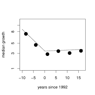
The coefficients of each model are the key result. The fixed effect gives the forest-wide response, which is the average growth of the species. It is thus not the same as the mean forest-wide growth, because the fixed effect weights each species equally.

The following graph uses the function fixef to get the parameters, then the function curve to add them to the graph. The points are forest-wide means, as graphed above.

3.1. Fixed effects.

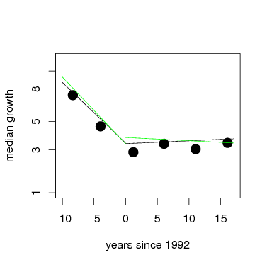
3.2. Repeated measures of individuals.

With lmer, accounting for the repeated measures of individual trees is easy to model. The tree tag, which identifies individuals, is added as a random effect. This is a fully nested model, individual within species. Here are the same two models as above, but now with tag added as a random effect. The graph overlays fixed effects from both models, with the model including tag in green.

3.3. Statistical signficance of the fixed effects.

Use the function display from the arm package to summarize the model results. All four models are displayed below.

The first section printed to the screen by display is the fixed effect, including both the coefficients (first column) and their standard error (second column). The term for time is how growth changed through time, negative numbers showing it declined. Confidence limits can be estimated by adding and subtracting 2 times the standard error. Display also repeats the model, to help keep track of which is which.

Whether or not tag was added to the model, the fixed effect of time shows that the average response was negative, and highly significantly so, over the first 3 census intervals. The models for census 3 and beyond, though, inclusion of tag alters the fixed effect: growth rate increased significantly when tag is not in the model, but adding tag changes the effect to slightly negative, though not significant. The graph above shows this; note that the differences are slight.

3.3.1. Model for census intervals 1-3, without tag.

3.3.2. Model for census intervals 1-3, with tag.

3.3.3. Model for census intervals 3-6, without tag.

3.3.4. Model for census intervals 3-6, with tag.

3.4. Individual species variation.

The real strength of lmer comes from the examination of how individual species vary. In the output of display, there are summary coefficients called Error terms. Each of these is a standard deviation across species: it measures how different species are.

Consider first the intercept in the first model, with tag included (the model named gmod1tag). The fixed effect, or average intercept of all species, is 1.38. But species differ, with standard deviation 0.39. Recall that most results fall within 2 standard deviations of the mean. This means that individual species have intercepts as high as 2.16 (1.38 + 2 × 0.39), and others as low as 0.60. Recall also that those are cube roots, since the model was run with CRGrowth.

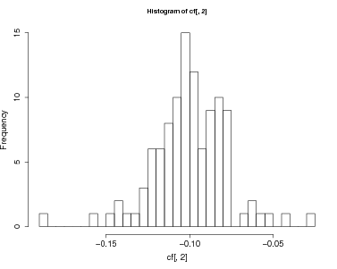
But the main point has been how growth rate varies through time, given as the time parameters. Under Error terms, the species effect for time is 0.026, and the fixed effect −0.0599. This means that the nearly the entire distribution of species responses falls < 0, meaning nearly all species had declining growth. In the second time interval (after census 3), species level variation was lower by a factor of 4.

There are additional Error terms for the tag, and a Residual term. The former shows variation among individuals within a species; notice it is approximately as high as the species term. The latter, Residual, is all remaining variation, which means variation in growth rates of individual trees in different census intervals, after accounting for the time effect. It is always higher than either species-level or individual-level variation, meaning most of the variance in growth is unexplained by the model.

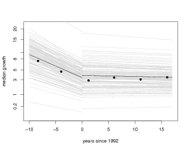
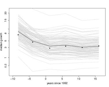
3.5. Individual species responses.

But lmer returns more: a set of coefficients for every species, and these make for direct interpretation. The function coef, also in the arm package, returns all coefficients. Here is graph overlaying every individual species onto the graph of fixed effects, using the models with tag included. The entire set of species coefficients are returned by coef(gmod1tag)$species; here I save those into a temporary variable called cf to reduce the amount of typing. There is a loop through every species, using the function curve to overlay one species’ results with a gray line. Since I chose to run models for two separate intervals of time, I repeat this for gmod1tag then gmod2tag. At the end, I add the fixed effects again, just as above, plus points for the forest-wide means.

Visually it is evident first that most of the variation between species is in the intercept term, while slopes of the lines are fairly consistent.

Coefficients can also be evaluated for individual species. Here are a few examples:

• Make a histogram of all growth responses to time
• Find the species with the biggest decrease in growth in the first interval
• Find the species with the highest growth intercept (growth in the very first census interval)

Other ideas to consider:

• Do species with higher initial growth show bigger changes in growth?
• Are species with lower growth rates more stable (less change through time)?
• Do saplings respond similarly to big trees (ie, repeat the model for dbh range 10-50 mm, or other sizes)?

4. Mixed model to assess species variation and temporal variation

An alternative model of growth change is to consider each census interval as a separate effect on growth, but without a linear change of growth through time. This would be reasonable if there is no a priori reason to expect steady increase (or decrease) in growth rate with time. Growth is allowed to vary from one census interval to the next, but can increase then decrease, etc.

The same function, lmer can be used, but now time is not a numeric variable, but simply a factor. The table already created, grate, has a column called censusfact, simply a number designating census intervals, but a factor, not an integer. Check this using R’s function str.

The coefficients are returned in the same way as they would be by R’s function lm. The intercept term is the estimated growth rate (cube root) in whatever census period comes first (in this case, censusfact=1). The remaining coefficients show the difference between growth in each of the other censuses and the first one. Thus, the intercept has to be added to the remaining coefficients in order to get the growth rate. The line with cf[,2:6] makes that adjustment, so that the temporary variable cf has the mean growth rates (root transformed) in each census period.

In the graph in which the x-axis is time, the responses will not be straight lines because the assumption of linear change has been removed.

Coefficients of every species can be evaluated to examine hypotheses about how growth differed between census intervals. For example, at BCI, the fixed effect of this model shows that the highest average growth was in the 1st interval, and species were extremely consistent about this: 115 of 117 had their highest growth rates in the first interval. The lowest average growth was the 5th interval, but the difference among intervals 3-6 was small, and species were much less consistent: 77 had their lowest growth rate in the 5th interval, but 11 did so in the 2nd and 16 others in the 3rd. Ten species’ lowest growth was in the final interval.

• How many species had their highest growth in the first census interval?
• How many species had their lowest growth in the last interval?
• Did growth rate in the first interval correlate with growth in the last?
• Do saplings respond similarly to big trees (ie, repeat the model for dbh range 10-50 mm, or other sizes)?

5. File Creation