CTFS Tutorials

• Tutorials: Top Level
• Server Use
• Growth changes
• Mortality changes
• Mortality vs. dbh
• Population Changes
• Biomass
• Growth vs. DBH
• ImageJ
• Plot maps
• Topography

Source file: http://ctfs.si.edu/ctfsdev/CTFSRPackageNew/files/tutorials/MortalityChange

Mortality changes

The question addressed here is how tree mortality has changed with time, in particular how species differ in the changes. There are two alternative models described:

• Mortality rate changing linearly with time
• Mortality rate varying from census to census, but not following a consistent change

Unlike growth analysis, mortality rates cannot be addressed with lmer, due to the variation in time interval among trees and among censuses. A proper mortality analysis must take this into account using a different death probability for every individual at every census. This can only be done with a Bayesian hierarchical model. The CTFSRPackage has a function lmerBayes which accomplishes the analysis. The Bayesian model has the advantage of producing complete confidence limits easily; the disadvantage is that it runs slowly. Analyses here on big datasets will take a couple hours to complete.

1. Formatting data

The calculations start with the full plot dataframes described at http://ctfs.arnarb.harvard.edu/Public/CTFSRPackage/help/RoutputFull.pdf. The BCI data can be downloaded from http://ctfs.arnarb.harvard.edu/bci/RAnalyticalTables after filling out the request form http://ctfs.arnarb.harvard.edu/webatlas/datasets/bci/.

In the CTFSRPackage, there are functions for loading data and calculating mortality rates. The function individual_mort.table in the demogchange topic collects results from several other functions to calculate mortality rates for individual trees and assemble them into a table in the format used by lmerBayes (which is the same format used by lmer. It is described in the Demography package.

The purpose is to create tables of mortality rates for every tree in every census interval. Choose any diameter category, and any set of censuses you wish to work with. Here is an example for big trees at BCI (dbh ≥ 400), with all seven censuses included.

The table mrate has one row per individual, and includes the tree’s tag number, coordinates, species, and dbh at the start of a census interval. The column census gives the census interval, so 1 means census 1 to 2, and 2 means census 2 to 3, etc. The column censusfact is the same, but as a factor variable instead of an integer. The time column is the mid-point of the interval between the two censuses, centered on 1992. This is the format needed by lmer and lmerBayes. The reason for centering time is that it is much better in linear regressions to have the x-axis near zero.

The column holding survival information is fate, TRUE for trees that survived the census interval; FALSE for the deaths.

2. Mean forest-wide mortality

First find the mean mortality rate of all individuals in each census period using the table mrate. This requires counting living and dead trees in each census, and there is a function calcMortIndivTable that does it, found with the DemogChange topic of the CTFSRPackage.

The same program also calculates the observed mortality rate for each species in each interval, saved below as spmort. Calls to tapply are also used to create a matrix of sample sizes: individuals per species at the start of each census interval, and number of survivors over each interval.

The time, meanyr, is the mean years since 1992 of each census interval.

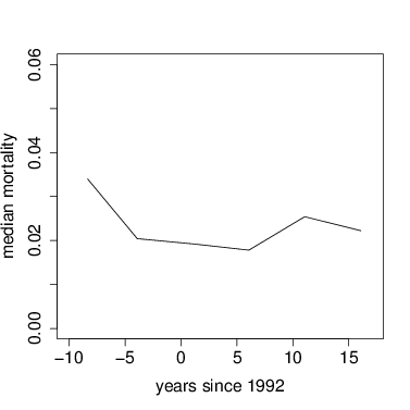
Graph median mortality vs. time.

3. Mixed model to assess species variation in linear changes through time

To test for changes in mortality rate, I have a model where the log(survival) is linearly related to time, that is log(survival) ≈ a+b*time. The two parameters, a and b, the intercept and slope, follow a Gaussian hyperdistribution across species. The function to produce predicted survival given this model is called lmerMortLinear and is found with the CTFSRPackage topic on demographic change.

The function lmerBayes is a Bayesian version of lmer found with the CTFSRPackage. It can fit mortality rate as a function of time, with species as a random effect; equivalent to a hierarchical model, where a Gaussian distribution describes the variation in species responses. The Bayesian version does not require a normal error, and it can account for differences in the census interval between trees and censuses.

Based on the shift in mortality that happened after the first 3 census intervals, I follow the approach of dividing the data into two periods, with censuses 1-3 and then 3-6. This approach should not necessarily be followed in other forests. Unlike growth, there is no tag effect; it’s not clear exactly whether there are repeated measures, since trees can only die once.

The calls to lmerBayes are complex, with many arguments. The data are defined in the first argument, exactly as in lmer. The arguments xcol, ycol, and randcol designate the predictors (xcol), the response ycol), and the mixed effect (randcol. They are quoted because they are character variables designating the names of the columns holding the required data. That’s how to write a formula in lmerBayes: in lmer, it would be written ycol   xcol + (xcol|randcol).

Note that there are two xcols because the time interval is needed to calculate annual mortality.

Subsequent arguments are controls for lmerBayes:

• start gives starting parameters for the fixed effect; they must be valid, and it is helpful if they are reasonably close to good answers
  the vector of starting parameters should give each a name
• model names the function used to calculate the response from the predictors
• startSD is not used in a binomial (ie, mortality) model, but something must be included
• startCov are starting estimates for the variance among species; it is helpful if they are reasonably close to a good result
• includeCovar=FALSE means estimate only the variances among species’ parameters, not their covariances
• badSDparam are not used in this model, but something needs to be included
• steps is how long to run the parameter search;
  • the example below has 2500 steps, which will produce good results
  • each took about 20 minutes on a good computer
  • one run will take an hour for saplings, where the sample is much larger
• burn is the number of steps to discard as burn-in; for runs of 4000 or more, it should be 1000
• showstep is how frequently to print intermediate search parameters to the screen

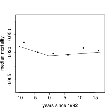
The coefficients of the models are the key result. The fixed effect gives the forest-wide response, which is the average mortality rate of all the species. It is thus not the same as the mean forest-wide mortality, because the fixed effect weights each species equally. The fixed effect is called bestmu, the error terms are in bestsigma, and species parameters are in best.

The following graph uses these to get the parameters, then the function curve to add them to a graph. The points are forest-wide means, as graphed above.

3.1. Fixed effects.

3.2. Statistical signficance of the fixed effects.

The Bayesian models return long chains of parameter values from which confidence limits can be calculated. For the fixed effects, they are in a table mu. A vector keep is used to exclude the burn-in steps. The CTFSRPackage function CI calculates 95% credible intervals.

The credible intervals show that In the first time period, census intervals 1-3, mortality declined significantly through time, since the intervals do not include zero. Over intervals 3-6, though, there was no significant change.

3.3. Individual species variation.

The error term from the Bayesian model is found in a matrix of covariance terms, bestsigma. In these models, only standard deviations were fitted, not the full covariance, so the off-diagonal elements are zero. Since the diagonal gives the variance, the square root is needed to show standard deviations.

Consider first the intercept in the first model. The fixed effect, or average intercept of all species, is -4.08. But species differ, with standard deviation 0.92. Recall that most results fall within 2 standard deviations of the mean, and that these are logarithms of mortality. These can be interpreted then to mean that individual species have mortality intercepts as high as 0.106 (10.6% y^-1), or exp(-4.08 + 2 × 0.92), and others as low as 0.0027 (0.27% y^-1), which is exp(-4.08 - 2 × 0.92).

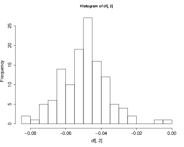
But the main point has been how mortality rate varies through time, given as the slope parameters. The species standard deviation for slope is 0.046, and the fixed effect -0.049. Considering again 2 standard deviations from the mean, the entire distribution of species responses overlaps 0, that is, though most species had declining mortality, quite a few showed increases.

3.4. Individual species responses.

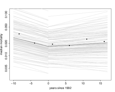
Like lmer, lmerBayes also returns a set of coefficients for every species, and these make for direct interpretation. The coefficients are in a table best. Here is graph overlaying every individual species onto the graph of fixed effects, using the models with tag included. First I save the coefficients into a temporary variable called cf to reduce the amount of typing. There is a loop through every species, using the function curve to overlay one species’ results with a gray line. Since I chose to run models for two separate intervals of time, I repeat this for mod1 then mod2. At the end, I add the fixed effects again, just as above, plus points for the forest-wide means.

Visually it is evident first that most of the variation between species is in the intercept term, while slopes of the lines are fairly consistent.

Coefficients can also be evaluated for individual species. Here are a few examples:

• Make a histogram of all mortality responses to time
• Find the species with the biggest decrease in mortality in the first interval
• Find the species with the highest mortality intercept (mortality in the very first census interval)

Other ideas to consider:

• Do species with higher initial mortality show bigger changes in mortality?
• Are species with lower mortality rates more stable (less change through time)?
• Do saplings respond similarly to big trees (ie, repeat the model for dbh range 10-50 mm, or other sizes)?

4. Mixed model to assess species variation and temporal variation

An alternative model of mortality change is to consider each census interval as a separate effect on mortality, but without a linear change of mortality through time. This would be reasonable if there is no a priori reason to expect steady increase (or decrease) in mortality rate with time. Mortality is allowed to vary from one census interval to the next, but can increase then decrease, etc.

The same function, lmerBayes can be used, but now time is not a numeric variable, but simply a factor. The table already created, mrate, has a column called censusfact, simply a number designating census intervals, but a factor, not an integer. Check this using R’s function str.

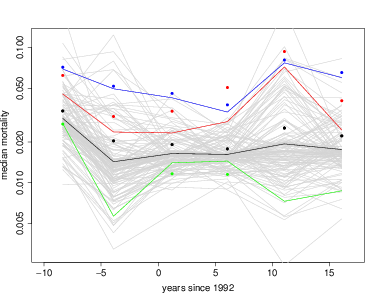
The table spmort created above can also be used to overlay observed mortality for individual species. In the graph below, blue points show observed rates for Trichilia tuberculata, and the blue line its fitted rates. The red shows the same for Dendropanax arborea and the green for Terminalia oblonga. In the case of Trichilia (blue), sample size was very large, so the fitted line is very close to the observed points. In the other two, sample sizes were much smaller, and the fitted lines are drawn toward the fixed effect. That’s always the way a hierarchical model works.

• How many species had their highest mortality in the first census interval?
• How many species had their lowest mortality in the last interval?
• Did mortality rate in the first interval correlate with mortality in the last?
• Do saplings respond similarly to big trees (ie, repeat the model for dbh range 10-50 mm, or other sizes)?

5. File Creation