CTFS Tutorials

• Tutorials: Top Level
• Server Use
• Growth changes
• Mortality changes
• Mortality vs. dbh
• Population Changes
• Biomass
• Growth vs. DBH
• ImageJ
• Plot maps
• Topography

Source file: http://ctfs.si.edu/ctfsdev/CTFSRPackageNew/files/tutorials/topography

Topography

R. Condit

The topography package includes just one file, solvetopo.r, whose purpose is estimating elevation data from survey data. This tutorial illustrates its use, and shows how to use the resulting elevation data to make a contour map. Creation of CTFS Plot elevation data in the standard CTFS format is demonstrated as well.

1. Formatting survey data

I assume that survey data are available in a format giving two locations and a vertical distance between the two. Here is a table of the survey data collected in the 49-ha Manaus plot. Two columns x1 and y1 give coordinates of one point, and x2 and y2 the coordinates of a second point. A sighting was taken from (x1,y1) to (x2,y2). The vertical distance between point 1 and point 2 is given in the column htdiff. The data are called manaus_topo_survey. To make it easier to follow commands with other data, I assign this to a table called simply survey; if you use the same name, you will be able to copy the commands below exactly.

2. Survey lines

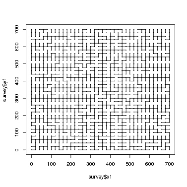
The survey lines can be mapped easilty in order to visualize the sightings taken. In order for the topography calculation to work, all points must be connected in one network of survey lines. If there are two (or more) separate networks, the solve.topo program will fail. Finding more than one network is a very common error in surveys, and it is easiest to detect using the graph illustrated here.

3. Data format for solve.topo

The function solve.topo requires the data table to be rearranged. Instead of x-y coordinates for the start and end survey points on each row, it requires a single identifier for each position. The function rearrangeSurveyData creates a table in this format. The table in the format described above is submitted as the only argument. The output of the function is a list including two different dataframe. One has every survey point with a new pointID and its coordinates; the second matches the input table, but with the point identifier instead of x-y coordinates.

The second of those two tables is submitted directly to solve.topo. There are other arguments to solve.topo, but if the output of rearrangeSurveyData is used, they can all be left at their default values.

Two arguments you might want to change, though, are baseelev and basept. The former is the elevation assigned to the point identified by the latter; defaults are 0 for the elevation and 1 for the base point. If one of the survey points has a known elevation, then use these two arguments to assign it.

All other elevations estimated by solve.topo are relative to this base point. For Manaus, I do not have the absolute elevation of any point, so I set point 1 to elevation 0 (which are the defaults).

4. Contours

The R function contours can be used to convert these elevations into a contour map. It requires, though, that there be a full grid of survey points. A CTFS plot survey usually has such a complete grid, and the Manaus data are complete. In the event you are lacking some points on the grid, there are tools in R’s GIS libraries that can be used to fill it in, but those are not covered here (there will be a CTFS R Package for GIS in the future).

To create a contour map, the new table elev created by solve.topo must be converted into a matrix.

The Manaus plot is 700x700 meters, with a survey point every 20 meters. So the grid (graphed above) is 36x36, and this is the size of the matrix to be created. Below are the calculations required for the Manaus plot. If you set plotdim to the size of your plot, the same calculations should work with no changes needed.

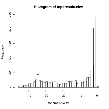
First combine the elevation results with the x-y coordinates, producing a table with x-y-z values. Below, I give that table the name coldata to emphasize that it has elevation data in column format, as opposed to the matrix format needed.

Next sort the table coldata by x and y (the Manaus data were not so ordered to begin with).

Then create the matrix matching the plot and grid size. The Manaus survey points are on a 20-m grid, hence gridsize=20; plotdim gives first the x then the y dimensions of the plot. The matrix matdata has as many columns as there are grid points along the x-axis, and as many rows as there are along the y-axis. In other words, the first column of the matrix has the elevations where x=0 (or x is at its minimum, if not 0). The first row of the matrix has the elevation at y=0 (or y is at its minimum, if not 0). This is the CTFS standard format for the elevation matrix!

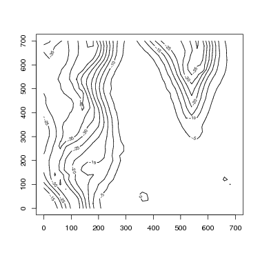
Now the R function contour produces the desired graph very easily. Notice that when the matrix is stored with columns representing the x-axis (as I just did), the transpose function t must be used. (It is a common problem at this point to get a contour graph that is a reflection over the line x=y of reality. If you follow the instructions here carefully, it will come out right.)

If you want to save contour lines, use the function contourLines. A future CTFS R Package in GIS will cover work with lines further.

A CTFS Plot Elevation object consists of both matdata and coldata. Other packages, particularly the map package, use elevation data in this format.

5. Sweave Output

HTML created by