CTFS Tutorials

• Tutorials: Top Level
• Server Use
• Growth changes
• Mortality changes
• Mortality vs. dbh
• Population Changes
• Biomass
• Growth vs. DBH
• ImageJ
• Plot maps
• Topography

Source file: http://ctfs.si.edu/ctfsdev/CTFSRPackageNew/files/tutorials/growthfitAnalysis

Growth vs. DBH

The following calculations in R run a model of AGB growth as a function of diameter, or as a function of agb, using a series of discrete size categories and a linear regression within each. The model presented here uses log(dbh) or log(agb) as the predictor (independent variable). The locations of the categories, or bins, of log(dbh) are not defined in advance, but are fitted as part of the model.

The R commands listed show all steps from loading data to running the model and graphing the output. All commands begin with >, and if continued on a second line, +. Comments between the commands describe the input and output of each.

The calculations start with the full data dataframes. These are described at
http://ctfs.arnarb.harvard.edu/Public/CTFSRPackage/help/RoutputFull.pdf, and can be downloaded from
http://ctfs.arnarb.harvard.edu/yourplot/RAnalyticalTables (of course you have to substitute a plot name for yourplot).

1. Source necessary functions

The following packages are necessary:

• growth.r
• growthfit.bin.r
• utilities.r
• statistics.r
• distributions.r

Running startCTFS will load these. The argument folder must match the location of the package on your computer.

2. Load plot data

Census data can be loaded using the function CTFSplot in utilities.r (or just attach the files). In the example here, there must be files bci.full5 and bci.full6 inside a folder full inside the listed path (so /home/fullplotdata/full/bci.full5 and same for bci.full6).

3. Calculate growth rates

3.1. Create a table of biomass growth rates using the function extract.growth.

The following creates a table of AGB increment for every individual with dbh≥100 mm. It excludes trees growing faster than 75 mm yr¹ (in dbh growth), or shrinking by 4 x the measurement error (which is 1 mm in small trees, 4-6 mm in big trees). Diameter is log-transformed (using logit=’x’). These are appropriate options for the calculations that follow. If you are worried about trimming the outliers, check the functions graph.outliers and graph.outliers.spp in order to see what is excluded. You need to change dbhunit to cm and maxgrow to 7.5 if your dbh is in centimeters, and set mindbh=10.

Of course you should submit census tables from your own plot instead of bci.full5 and bci.full6.

Note that I occasionally use if(!exists). You can ignore these when executing functions. I use it to prevent certain long-running commands from repeating every time I test the calculations. In this case, once agb.growth is created, it won’t be created again.

3.2. Graphing growth rate.

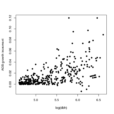
This extracts growth for just one species. You might also make a graph of all growth rates at once in order to explore the data.

---

---

4. The model

4.1. Fitting.

Here is how to fit the model for just a single species, then graph the result. The table onespdata produced above has growth data from a single species that is appropriate for the function. For testing, you can start by using method=optim, since it produces the fit faster, but optim does not produce confidence limits, so use method=Gibbs for final results.

Here, dbh is used as the predictor in the model, but this can be changed by setting sizecol=’agb’ instead of dbh.

The option nobin sets how many dbh categories will be used. Here it is set to 2, so just one division point will be estimated. (The location of the division point will be optimized, but the number of division points must be set at the start.)

The option sdmodel defines the model used for related SD to log(size). The default is linear.model.ctr, simply a straight line with intercept defined at the mid-point of the x axis. The number of parameters for the SD model, defined by startsd, must match the number of parameters expected by sdmodel: 2 parameters for a linear model. The second run here (fit2) illustrates a model with 3 parameters, where the SD is constant below a certain value of x, then increases linearly. This allows the SD to increase rapidly at large size while remaining positive at small size.

4.2. Model output.

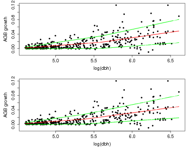
The output of the model was saved in the variables fit and fit2, which are lists that include a lot of information. The element fit$model includes the original data (fit$model$x and fit$model$y), plus the fitted value for each (fit$model$pred), and also the fitted SD at every point (fit$model$predSD). The best fit model parameters are fit$best, and confidence limits in fit$CI. The best fit standard deviation parameters are in fit$bestSD. (The model assumes a linear increase in the standard deviation around the line, and the two SD parameters describe the linear increase.)

---

---

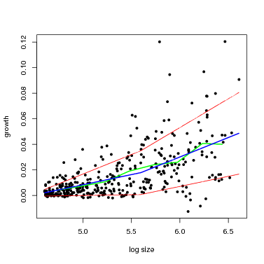
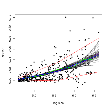
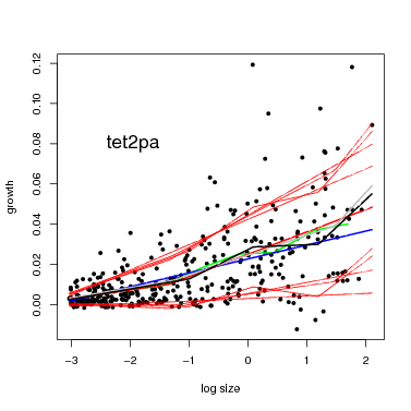
There is a function graph.growthmodel.spp that handles the graphing in a single step. It graphs the points for individual trees, and adds the fitted model in blue (you can change the color). A green line shows the mean growth in 10 equally-spaced divisions (from graphdiv=10). There is also an option to overlay alternative model fits as a way of visualizing statistical confidence in the model, illustrated in the second example below (conf=50): 50 different gray lines are drawn using randomly selected parameters from the Gibbs sampler used to fit the model (all the parameters are returned in fit$fullparam). An advantage of the Gibbs sampler is this way of showing confidence: every set of parameters returned (after the burnin) can be considered equally good fits to the model.

Note that confidence in the model is different than the standard deviation (yellow lines in the previous figure). The latter gives variation among individuals, but the gray lines provide an estimate of confidence in the position of the blue line.

At small dbh (remember, though, only dbh≥ 100 mm are included), the SD is small, meaning little variation among individuals, and the confidence bands are narrow. Both SD and the confidence bands spread at larger size.

---

---

---

---

4.3. Interpreting the parameters.

The parameters provided by fit$best describe the model. The first parameter is the break point between the two bins, and the best estimate is 6.04 for in the example here for Tetragastris. The next two parameters are the two slopes, first before the break point, then after the division. In this case, the best fit for them is 0.017 and 0.039, so the slope gets steeper, and both are significantly > 0 (since the confidence intervals do not reach 0). But the two slopes are not significantly different from each other, since their confidence limits overlap. The last parameter is the intercept parameter, which is the estimated growth in the middle of the middle bin.

4.4. Comparing results for different number of bins.

The interesting result is whether using three or four bins improves the model. The function run.growthfit.bin automates the process of running the model 4 times, with 1 through 4 bins. One bin is just a standard linear model; I have not yet tried 5 or more bins.

The following example runs the Gibbs sampler for 1500 repetitions (noreps=1500). In final fits, I recommend using noreps=5000. But for illustration here, the 1500 steps provide adequate parameter values. The variable fitlist creates a list with just one entry, named for the species’ code tet2pa. This is how the data are passed to the graphing function.

The funtion overlay.growthbinmodel makes a graph of all 4 models. It expects the fit to be a list, which is why I created fitlist. The first option below shows the graph on the screen; the second exports the graph as a pdf (export=pdf ).

---

---

4.5. Fitting the model for all species.

The next step is to run the fit for all species in a plot. Here I limit the selction to species with at least 40 individuals total and 15 individuals ≥300 mm dbh. You may wish to change the limits, but the fitting procedure requires ≥5 individuals per category, so it will fail with species having < 20 individuals above 100 mm dbh.

This will run the Gibbs sampler 5000 steps per species, and will take 10-20 hours to complete. Note that the example here uses agb as the predictor by submitting size=’agb’.

The output, saved in the object linearbin.fit.allspp, is a list, one element per species. Each element has four subelements, one per the models with 1-4 bins. Each of those subelements is a single model fit, with all the elements described above.

The object linearbin.fit.allspp can be passed directly to the function overlay.growthbinmodel to graph results for all the species. In the first example, export=NULL and the graphs are printed to the screen. In the second example, export=pdf and a pdf with all the graphs is created. You can change the file name to whatever you please using outfile.

4.6. Statistical comparison of the models.

Finally comes a statistical test for assessing the 4 different models (1-4 bins) for each species. The function compare.growthbinmodel calculates the best model using the AIC, or Akaike Information Criteria, and makes a graph of this model.

It also produces a list of 3 different tables:

1. The first gives the slope of the growth vs. AGB regression in each bin of the best model. There are up to four slopes per species.
2. The second gives the lower 95% confidence limits (or credible intervals in Bayesian terminology) for those same slopes.
3. The third has upper credible intervals.

The results from 37 species at BCI are shown below. The columns with NA indicate those slopes were not needed in the best fit, that is, if there is only one slope, then the best model used only one bin, etc. Any negative slope means growth rate declined with size in that size bin. If the upper credible interval is also negative, then the slope is significantly < 0. At BCI, only quaras, Quararibea asterolepis, had a significant decrease in growth rate in the largest size category. Brosimum alicastrum (brosal) and Prioria copaifera (pri2co). had declines, but not significantly so. Poulsenia armata (poular) had a peculiar fit, with a decline in growth in the second to last category, but an increase in the last. Poulsenia was the only species for which all 4 bins were needed, and only 3 other species required 3 bins. More than half the species (20 or 37) were best modeled using a straight line.

Estimated slopes in AGB bins for BCI species, based on the model with the highest AIC.

Upper confidence limits for slopes in AGB bins. Any of these < 0 indicate a slope significantly less than zero. There are also lower confidence limits (not shown), and any of those > 0 indicate a significantly positive slope.

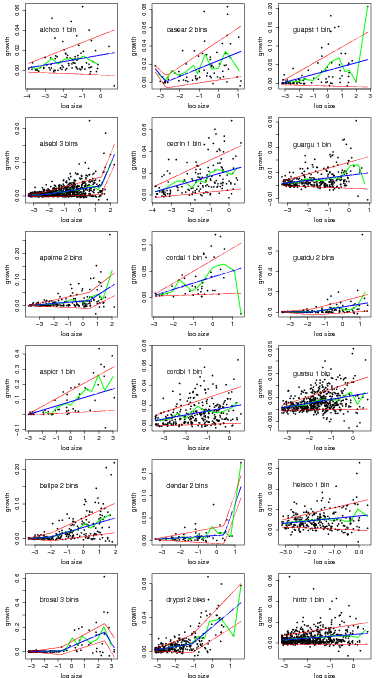
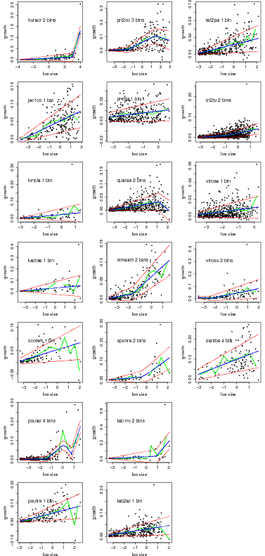
Graphs of the best model based on AIC for all species.

---

---

---

---

Now use a run with an updated trimming of extreme growth, permitting more negative growth (see trimGrowth), and the alternative model of SD where the slope can turn upward at large size.

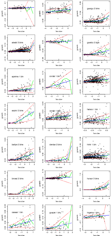
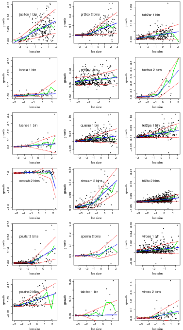
Graphs of the best model based on AIC for all species.

---

---

---

---

You can also export all the graphs at once into a single pdf to a file named by outfile.

5. File creation

Anyone intereted in seeing how Sweave works in R to create this document can contact me.