CTFS Tutorials

• Tutorials: Top Level
• Server Use
• Growth changes
• Mortality changes
• Mortality vs. dbh
• Population Changes
• Biomass
• Growth vs. DBH
• ImageJ
• Plot maps
• Topography

Source file: http://ctfs.si.edu/ctfsdev/CTFSRPackageNew/files/tutorials/abundFitModel

Population Changes

The question addressed here is how much abundances of all the tree species in a plot fluctuate from census to census. At one extreme, abundances are stabilized, and populations do not change. In contrast, there may be environmental drivers favoring some species and not others, so that some species show marked (ie, more than neutral) increases and others decreases. In between the two extremes is a community in which no external drivers affect abundances but populations fluctuate due to demographic stochasticity: a neutral forest.

The test of these models hinges on a histogram of the rate of population change of every species in the forest. Define λ = , the ratio of a future population N₁ to the current N₀, and r = little.r = logλ. In a highly stabilized community, λ ≈ 1 for every species, and r = 0, whereas in a forest with environmental fluctionas, λ may be distributed widely but ought to be centered close to 1. The neutral community would fall in between, with λ varying a small amount due to chance alone.

The distribution of λ and r under neutrality can be predicted mathematically, assuming deaths are binomially distributed across individuals and a Poisson distribution of births whose mean matches the death rate. Because of this statistical model of neutral fluctuations, any environmentally caused variation can be estimated precisely. In a conceptual sense, it means subtracting the predicted neutral variance of λ from the observed variance of λ; what’s left is the environmental variances. The neutral prediction depends on the mortality rate, which is also fitted by the model. The following demonstrates an R program for running this model with forest plot abundances.

The model allows various functional forms for the distribution of population growth. The example below is based on a power probability distribution, where p(x) ∼ x + 1^k (k < −1). The exponent k describes how broad the distribution, with more extreme k (ie, more negative) meaning a narrower distribution. Indeed, frac1k is close to the standard deviation of the distribution of r. The power distribution, though, allows k on the negative size of x to differ from k for x positive. It is thus an asymmetric power distribution.

1. Formatting data

The calculations start with the full plot dataframes described at http://ctfs.arnarb.harvard.edu/Public/CTFSRPackage/help/RoutputFull.pdf. The BCI data can be downloaded from http://ctfs.arnarb.harvard.edu/bci/RAnalyticalTables after filling out the request form http://ctfs.arnarb.harvard.edu/webatlas/datasets/bci/. Assume for the following example that dataframes for three censues are loaded, bci.full1, bci.full2, and bci.full3. A species table, such as bci.spptable, is also needed. The species table has a column IDlevel that indicates which taxa are neither valid species nor valid morphospecies – cases where a species code includes a mixture of unknown species. The typical example of these mixtures are unidentified trees, with codes such as UNID or uniden. They must be excluded from the analysis, since changes in abundance of those species codes do not represent population fluctuations of a species.

2. Running the model of environmental variance

A function in the CTFSRPackage (topic population change) called model.littleR.Gibbs runs the model to estimate leftover environmental variance over two census intervals. To run with your own data, simply replace census1 and census2 with your own R Analytical Tables for a CTFS plot. The fitting procedure requires a Bayesian parameter-search, which must run at least 1000 steps. I recommend here running the model once for 1200 steps, as in the example below in order to explore results. In order to get really solid parameter estimates, a run of 10,000 steps should be set. Ddepending on your computer, 1000 steps should take about 3 minutes and 10,000 steps 30 minutes. Note that mindbh needs to be set. The example below assumes dbh is in mm, and is set to 10.

3. Model results

The result, saved object as mod, is a Bayesian model object including the estimated parameters and their confidence, plus the complete parameter search. The element of the list mean has the fitted parameters. The first two describe the estimated distribution of mortality rates:

• hyperMu = mean of the log(mortality) rate across species;
• hyperSD = standard deviation of the log(mortality) rate across species.

The next three parameters describe the distribution of population growth rates, as defined by r = logλ:

• hyperR = mean of r across species, generally very close to 0;
• hyperSDlow = inverse of the exponent of the power distribution for x < 0; its negative is similar in magnitude to the median population population change of those species declining in abundance;
• hyperSDup = IBID for the positive half of x; its negative is similar in magnitude to the median population population change of those species increasing in abundance.

Upper and lower confidence limits for the five parameters are returned in the components upper and lower.

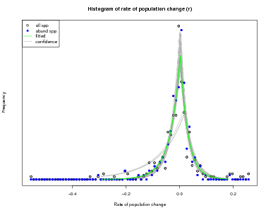
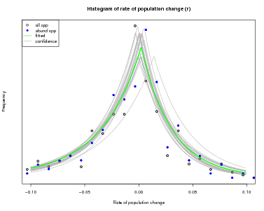
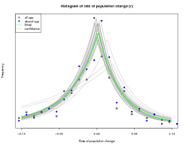
There is another function in the same topic of the CTFSRPackage called graph.abundmodel that creates a graphical view of the fitted model. Pass it the name of the model object and nothing more and it will show a histogram of observed rates of population change r (open circles for all species, blue circles for abundant species), along with the fit to the histogram (green line).

The green curve is the estimated variation in in abundance due to the environment: what is left over after stochastic demography is accounted for. The points, which give the observed histogram, include stochastic plus environmental, thus should be broader than the green curve.

The x-limits of the graph can be adjusted using the argument xrange. In addition, confidence limits can be added by setting conf=50, or any other positive number (the number of lines to draw). The confidence lines are based on all the steps in the Bayesian sampling and reflect confidence in the fitted model.

4. Running the model for several censuses

There is a wrapper function fitSeveralAbundModel that can handle any number of census datasets. It simply fits the abundance model for each pair of censuses, then for the first and last census, saving all into one big list, plus it repeats all the models for larger trees, setting mindbh to 10 times the submitted value. It’s only purpose is to finish a series of models from one plot in a single model run. Since it takes about 30 minutes per census, you might leave it running overnight. The following code saves the results to an R data object in the folder abunddist.