CTFS Tutorials

• Tutorials: Top Level
• Server Use
• Growth changes
• Mortality changes
• Mortality vs. dbh
• Population Changes
• Biomass
• Growth vs. DBH
• ImageJ
• Plot maps
• Topography

Source file: http://ctfs.si.edu/ctfsdev/CTFSRPackageNew/files/tutorials/map

Plot maps

R. Condit

The map package includes functions for creating maps of tree distributions in CTFS plots. All functions are in a single file, map.r. There are functions for drawing single maps, on which one or more species can be included, and one or more dbh classes. And there are functions to create many maps, for example of every species in a plot. The functions have many options for adjusting features (point size, colors), and allow maps to be drawn on the screen or exported as various graphics file types. All functions use input data in the standard web/data_formatCTFS format. Most use data in the split format, so having R objects in this format saved already is convenient.

This tutorial illustrates use of 4 of the functions, map, pdf.allplot, png.allplot, and complete.plotmap

1. Loading data

The web/data_formatutilities function</a> can be used to attach an existing split data object for a single census. Otherwise, load such an object. In the example below, the object bci.split6 is attached. It is a list of dataframes, with one dataframe per species; at BCI there are 326 species, and the first 6 are listed below, as 6-letter mnemonics.

2. The basic map function

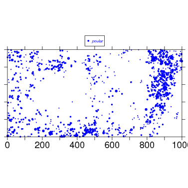
This is the core function. It will create a single map of one or more species, with many options available for adjusting the map.

The simplest use requires identifying the split data object to use, here bci.split6, and a species mnemonic, which of course must be one of the names in the object. (The default plot size is 1000x500 m, so if your plot is 25 ha, you will have to set plotdim=c(500,500).)

To begin tweaking the map, check the arguments, and also read about them at the web/data_formatmap help page. There are a lot of arguments.

To make a larger map, use the arguments ht and wd to set the overall height and width of the graph (inches), and plotside to set the width of plot itself. To use these parameters, you have to set export="windows", export="mac", or export="unix", depending on your operating system. I use the latter.

> map(splitdatafile=bci.split6,species=’poular’,wd=11,ht=8,plotside=10,export=’unix’)

To export a map, use export=’pdf’ and set the output using filepath and outfile

> map(splitdatafile=bci.split6,species=’poular’,wd=11,ht=8,plotside=10,export=’pdf’,filepath=’maps/’,outfile=’PoulseniaMap’)

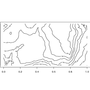
3. Topo lines

The most appealing maps include topo lines. This requires elevation data in matrix format, a standard format for CTFS plots (data for most plots are available at http://ctfs.arnarb.harvard.edu/Public/Datasets/CTFSTopography/). I have BCI data in CTFSElev_bci, and below I save the matrix portion as bci.elev. The matrix has 201 columns, one every 5 m of the 1000-m plot, and 101 rows for the 500-m axis. The tutorial on topography desribes this format (http://ctfs.arnarb.harvard.edu/Public/CTFSRPackage/index.php/web/tutorials/topography/index.html.

The R function contours uses data in this matrix format to map contour lines. Since the plot is 1000x500 m, use par to set the size of the figure so that it is twice as wide as long.

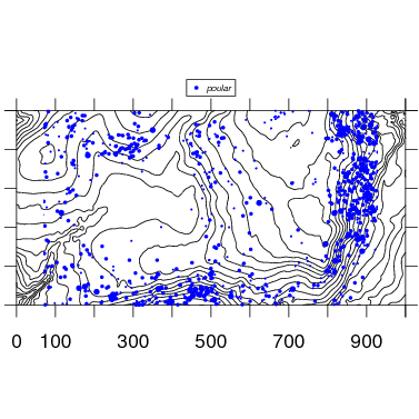
The map function makes use of contour to add topo lines to the species map. Below is the map with default options. Changing the size or exporting would be identical to the examples above.

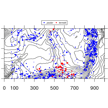
4. Multiple species

Two or more species are mapped by simply adding species names. Check options for color and symbol size and shape to refine.

5. Multiple maps

There is a function pdf.allplot that automatically generates a set of pdf maps for all species in a plot. This example uses a table of species names to include Latin names; most CTFS plots have species tables available at their own database web sites (for BCI: http://ctfs.arnarb.harvard.edu/bci/RAnalyticalTables). Be sure to adjust plotdim to the size of your plot, and you will have to experiment with the size of the graph by adjusting plotside, h, and w.

«» head(bci.spptable)[,1:5] This creates a single pdf with 326 pages, a map for each species:

This creates 326 pdfs, one separate file for each species:

There is an equivalent function, png.allplot, that creates 326 separate maps in png format.

6. Full stem map

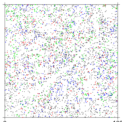
One function, complete.plotmap, makes a map of every individual of all species in black dots. Then it overlays a few individual species in different colors. The map can be any rectangular portion, or the entire plot, based on the options xrange and yrange.

The basic use draws a map of all individuals, then overlays the 3 most common species in green, blue, and red, in a 100x100 m section of the plot.

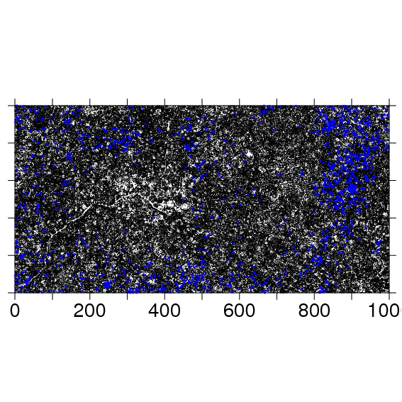
To make a full plot map, it is useful to make ptsize very small. The stream in the southwest corner of the BCI plot is evident in the stem map.

The following code exports the same map as a pdf to the file named:

Output created by